Loading...
Building a Neural Network from Scratch with Python & NumPy
08/27/2024
Summary
A beginner-friendly guide to neural networks: from individual neurons to a complete Python model that predicts house prices using NumPy.
Introduction
Artificial Intelligence is transforming our world, and at its core are neural networks. In this article, we’ll break down how these powerful systems work, from the neurons to the complete network. We’ll even build a simple model in Python, so you can experience AI firsthand. Let’s dive in!
A single neuron
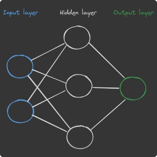
If you are already a bit familiar with AI, you probably already saw an illustration like the one below, otherwise no problem. This illustration shows a simple neural network, which we’re going to inspect and implement today from scratch in Python. The neural network is the fundamental concept behind modern AI and it’s a really interesting topic to study. But before dive into the code, let’s first focus on the key concepts behind the network.

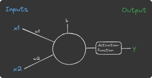
To better understand how a neural network works, let’s first zoom in on a single node (neuron):
Imagine we have a motion detector in our garden that turns on the light when it detects motion and when it's dark. Additionally, there's a dial that lets us set a value to make it harder or easier to turn on the light. This motion detector is an abstract representation of a single neuron. In a neural network, the detected motion and surrounding light are the inputs (x1 and x2). These inputs are connected to the neuron through weights, which determine how much each input influences the result. The dial in our example represents the bias, an additional independent value that adjusts the impact of the inputs on the final result. To calculate the neuron's output, we multiply each input (x1, x2) by its corresponding weight (w1, w2). We then sum all these products and add the bias. This gives us a numerical value that represents the neuron's response. In older neural models, this value indicated whether the neuron "fired" (light on) or didn't "fire" (light off). Since this approach only allowed for two states (1 or 0), it was later decided to use an activation function to provide a probability of how strongly the neuron "fires," usually resulting in a value between 0 and 1. In our case, we use the sigmoid function, which is very popular in such networks.
→ formula of the sigmoid function: σ(z) = 1 / (1 + e^(-z)) → final formula: y = σ(w1x1 + w2x2 + b)

A neural network
Okay, now we looked at the functionality of one single neuron. To build a network we simply put multiple of them together into layers and connect the different layers that the output of the first layer is the input of the second layer and so on.
Our simple neural network consists three different layers:
1. Input Layer: Receives initial data (e.g., house size and age), the neurons here aren’t real neurons, just some normalized numbers, which represent the input
2. Hidden Layer(s): Processes information
3. Output Layer: Produces the final result (e.g., house prize)
To wrap it up let’s look a bit closer on the dataflow in a neural network by looking at an example.
1. Input values enter the network through the input layer. (e.g., the normalized house size is 0.8 and the normalized age is 0.4, so one input neuron has the value of 0.8 and the other of 0.4)
2. Each hidden neuron receives all input values (e.g., 0.8 and 0.4).
3. Hidden neurons calculate the inputs and pass outputs to the output layer.
4. The output layer calculates the final result based on hidden layer outputs.
We will look at this later a bit closer and implement it into our code.Let’s first of all create a class with the structure of our neural network in Python:
import numpy as np

class NeuralNetwork:
    def __init__(self, input_size, hidden_size, output_size):
        self.input_size = input_size
        self.hidden_size = hidden_size
        self.output_size = output_size

        # initialize random weights and biasses
        # W1 and b1 are between the inputlayer and the hiddenlayer
        self.W1 = np.random.randn(self.input_size, self.hidden_size)
        self.b1 = np.ones((1, self.hidden_size))

        # W2 and b2 are between the hiddenlayer and the outputlayer
        self.W2 = np.random.randn(self.hidden_size, self.output_size)
        self.b2 = np.ones((1, self.output_size))

# create network
nn = NeuralNetwork(input_size=2, hidden_size=3, output_size=1)Introduction to training
Now that we've created the structure of the network, let's move to the next step called "training". The following overview shows a single training step, normally we train in multiple batches and many rounds. It works as follows:
- Initialization:We have a network initialized with random weights and biases.
- Forward pass:We take the training data, which consists of input and correct output. We feed the input into the neural network and compute the predicted output.
- Cost Function:We then compare this predicted output to the correct output using a cost function, which shows the "size" of the mistake the network produces. There are many different cost functions, but for our example we use one called Mean Squared Error (MSE).
- Backward pass:We take this cost to go backwards through the network and use partial derivatives to calculate how every weight and bias needs to be updated.
- Update:Finally, we update every weight a little bit in the correct direction. The parameter learning rate tells the system how big the steps should be when it updates the weights and biases.
Forwardpass
As briefly explained in the previous section, the forward pass takes the values of the provided data, feeds them into the network, and calculates the output. I think an example can explain this better than any words. So let's dive in!
1. The Situation: In our example, we have two input parameters: the size of a house (i1) and the age of the house (i2). Our goal is to train a neural network that can predict the price of the house (o1) based on these two parameters. For our training, we use this simple training set:
# [size, age]
X = np.array([
    [100, 5], [120, 10], [80, 15], [150, 2], [90, 20],
    [110, 7], [95, 12], [130, 8], [140, 5], [75, 18],
    [85, 14], [125, 6], [100, 10], [135, 4], [105, 9],
    [115, 11], [140, 3], [80, 20], [90, 22], [120, 14]
])

# price in t€
y = np.array([
    [200], [220], [170], [280], [160],
    [210], [175], [225], [270], [155],
    [185], [230], [195], [265], [175],
    [215], [275], [165], [185], [225]
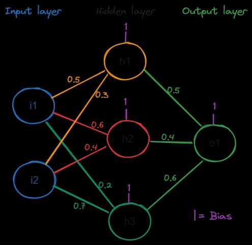
])2. First, we initialize the network with some random weights and biases. In the illustration, I always used 1 as bias for simplicity.

3. Then we need to normalize our data so that every data point has the same influence on the network. I won't explain this explicitly, but if you want to understand this step, please search for it online. There are many great explanations available. For our example, we take the values of the first input [100, 5], which are normalized and rounded to -0.3 (i1) and -0.8 (i2).
4. With these inputs and our weights and biases, we're now able to calculate an output. a) We calculate the result for each hidden neuron with the sum I showed earlier: h1 = σ(-0.3*0.5 + (-0.8)0.3 + 1) = σ(0.61) = 0.65 h2 = σ(-0.30.6 + (-0.8)0.4 + 1) = σ(0.5) = 0.61 h3 = σ(-0.30.2 + (-0.8)*0.7 + 1) = σ(0.38) = 0.59 b) Based on the results of the hidden layer, we calculate the result of the output layer: o1 = σ(h10.5 + h20.4 + h30.6 + 1) o1 = σ(0.650.5 + 0.610.4 + 0.590.6 + 1) o1 = σ(1.923) = 0.87
Alright, now that we have a solid overview of the forward pass: Let's code!
import numpy as np
# sigmoidfunction
def sigmoid(x):
    return 1 / (1 + np.exp(-x))

class NeuralNetwork:
    def __init__(self, input_size, hidden_size, output_size):
        self.input_size = input_size
        self.hidden_size = hidden_size
        self.output_size = output_size

        # initialize random weights and biasses
        # W1 and b1 are between the inputlayer and the hiddenlayer
        self.W1 = np.random.randn(self.input_size, self.hidden_size)
        self.b1 = np.ones((1, self.hidden_size))

        # W2 and b2 are between the hiddenlayer and the outputlayer
        self.W2 = np.random.randn(self.hidden_size, self.output_size)
        self.b2 = np.ones((1, self.output_size))

    # Forwardpass
    def forward(self, X):
      # calculate the output of the hidden layer
      self.z1 = np.dot(X, self.W1) + self.b1
      self.a1 = sigmoid(self.z1)

      # calculate the output of the output layer
      self.z2 = np.dot(self.a1, self.W2) + self.b2
      self.a2 = self.z2

      return self.a2

# create network
nn = NeuralNetwork(input_size=2, hidden_size=4, output_size=1)Backwardpass
Once we’ve calculated the output for a given input, we often find it’s not as accurate as we’d like. Fortunately, the backpropagation algorithm allows us to improve our results. This powerful method works backwards through the network, starting from the error, to calculate the loss for each neuron. With this information, we can adjust weights and biases incrementally to minimize the error and improve the output.
At its core, backpropagation uses partial derivatives to determine how each input affects the final error. This concept is similar to analyzing the impact of inputs x₁ and x₂ on the final error in a single neuron or perceptron. The algorithm follows a series of steps: first, it performs a forwardpass to calculate the output; then it computes the error by comparing the output to the expected result. Next, it propagates this error backwards through the network, calculating gradients along the way. Finally, it updates the weights and biases to reduce the error.While I won’t delve into the mathematical details of backpropagation here, those interested in a deeper understanding might find 3Blue1Brown’s YouTube video on the subject helpful. However, to give you a practical sense of how this works, here’s a simplified Python implementation of the backward pass in a neural network:
import numpy as np

# sigmoidfunction
def sigmoid(x):
    return 1 / (1 + np.exp(-x))

# define the derivative of the sigmoid function
def sigmoid_derivative(x):
    return x * (1 - x)

class NeuralNetwork:
    # ...

    def backward(self, X, y, output, learning_rate):
      m = X.shape[0]

      # Compute the error term for the output layer
      self.error = y - output
      self.delta_output = self.error

      # Compute the gradients for W2 and b2
      self.W2_grad = np.dot(self.a1.T, self.delta_output) / m
      self.b2_grad = np.sum(self.delta_output, axis=0, keepdims=True) / m

      # Compute the error term for the hidden layer
      self.error_hidden = np.dot(self.delta_output, self.W2.T)
      self.delta_hidden = self.error_hidden * sigmoid_derivative(self.a1)

      # Compute the gradients for W1 and b1
      self.W1_grad = np.dot(X.T, self.delta_hidden) / m
      self.b1_grad = np.sum(self.delta_hidden, axis=0, keepdims=True) / m

      # Update the weights and biases using gradient descent
      self.W2 += learning_rate * self.W2_grad
      self.b2 += learning_rate * self.b2_grad
      self.W1 += learning_rate * self.W1_grad
self.b1 += learning_rate * self.b1_gradTraining and testing
After defining our neural network architecture, we train and test it using a dataset of house prices. This process involves several key steps:
1. Initializing the Network: We create an object of our neural-network-class object with 2 input neurons, 4 hidden neurons, and 1 output neuron.
2. Dataset: We then define our dataset, where X represents the input features (size and age) and y represents the target values (house prices in thousands of euros).
3. Normalization: we normalize the data to ensure all features are on a similar scale, which helps the network learn more effectively.
4. Training: The training process occurs over 2,000 epochs with a learning rate of 0.05. In each epoch, we perform a forwardpass through the network, followed by a backward pass to update the weights and biases. We calculate the mean squared error (MSE) as our loss function and print it every 100 epochs to monitor the training progress.
5. Prediction Function: We define a predict function that takes a house’s size and age as inputs, normalizes them using the same parameters as our training data, feeds them through the network, and then denormalizes the output to get the predicted price in thousands of euros.
6. Testing: We test our trained network by predicting prices for hypothetical houses.
This example illustrates the complete process of creating, training, and using a simple neural network for regression tasks, showcasing the practical application of the backpropagation algorithm we discussed earlier.
import numpy as np
import matplotlib.pyplot as plt
#
# sigmoidfunction
def sigmoid(x):
    return 1 / (1 + np.exp(-x))

# define the derivative of the sigmoid function
def sigmoid_derivative(x):
    return x * (1 - x)


class NeuralNetwork:
    def __init__(self, input_size, hidden_size, output_size):
        """        """
        self.input_size = input_size
        self.hidden_size = hidden_size
        self.output_size = output_size

        # Weights and biases
        self.W1 = np.random.randn(self.input_size, self.hidden_size)  # Weights between input and hidden layer
        self.b1 = np.ones((1, self.hidden_size))  # Biases for the hidden layer
        self.W2 = np.random.randn(self.hidden_size, self.output_size)  # Weights between hidden and output layer
        self.b2 = np.ones((1, self.output_size))  # Biases for the output layer

    # Forward Pass
    def forward(self, X):
        """        """
        self.z1 = np.dot(X, self.W1) + self.b1  # Linear combination for hidden layer
        self.a1 = sigmoid(self.z1)  # Apply activation function to hidden layer
        self.z2 = np.dot(self.a1, self.W2) + self.b2  # Linear combination for output layer
        self.a2 = self.z2  # Output layer (no activation for regression)
        return self.a2


    def backward(self, X, y, output, learning_rate):
        """        """
        m = X.shape[0]  # Number of training examples

        # Error and delta calculations
        self.error = y - output  # Error at the output layer
        self.delta_output = self.error  # Delta for the output layer
        self.error_hidden = np.dot(self.delta_output, self.W2.T)  # Error at the hidden layer
        self.delta_hidden = self.error_hidden * sigmoid_derivative(self.a1)  # Delta for the hidden layer

        # Gradient calculations
        self.W2_grad = np.dot(self.a1.T, self.delta_output) / m
        self.b2_grad = np.sum(self.delta_output, axis=0, keepdims=True) / m
        self.W1_grad = np.dot(X.T, self.delta_hidden) / m
        self.b1_grad = np.sum(self.delta_hidden, axis=0, keepdims=True) / m

        # Update weights and biases
        self.W2 += learning_rate * self.W2_grad
        self.b2 += learning_rate * self.b2_grad
        self.W1 += learning_rate * self.W1_grad
        self.b1 += learning_rate * self.b1_grad

# create a networkobjekt
nn = NeuralNetwork(input_size=2, hidden_size=4, output_size=1)

# define data
# [size, age]
X = np.array([
    [100, 5], [120, 10], [80, 15], [150, 2], [90, 20],
    [110, 7], [95, 12], [130, 8], [140, 5], [75, 18],
    [85, 14], [125, 6], [100, 10], [135, 4], [105, 9],
    [115, 11], [140, 3], [80, 20], [90, 22], [120, 14]
])

# Price in thousand euros
y = np.array([
    [200], [220], [170], [280], [160],
    [210], [175], [225], [270], [155],
    [185], [230], [195], [265], [175],
    [215], [275], [165], [185], [225]
])

# normalize data
X_mean, X_std = X.mean(axis=0), X.std(axis=0)
y_mean, y_std = y.mean(), y.std()

X_normalized = (X - X_mean) / X_std
y_normalized = (y - y_mean) / y_std

# Training loop
epochs = 2000
learning_rate = 0.01
losses = []

for epoch in range(epochs):
    # Forward pass
    output = nn.forward(X_normalized)

    # Backward pass
    nn.backward(X_normalized, y_normalized, output, learning_rate)

    # Calculate and print loss
    mse = np.mean(np.square(y_normalized - output))
    losses.append(mse)
    if epoch % 100 == 0:
        print(f"Epoch {epoch}, Loss: {mse}")

# Prediction function
def predict(size, age):
    """    """
    input_normalized = (np.array([[size, age]]) - X_mean) / X_std
    output_normalized = nn.forward(input_normalized)
    return output_normalized * y_std + y_mean

plt.plot(losses)
plt.xlabel("Epoch")
plt.ylabel("Loss")
plt.title("Loss while training")
plt.show()

# Test Prediction
print("\nPredictions:")
print(f"House with 110 m² and 7 years: {predict(110, 7)[0][0]:.2f} t€")
print(f"House with 85 m² and 12 years: {predict(85, 12)[0][0]:.2f} t€")Result
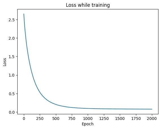
The chart down below shows how our neural network model got better at predicting house prices as it learned. At the start, it made lots of mistakes (high loss). But as it practiced more and more (more epochs), it made fewer and fewer mistakes. The line on the chart goes down quickly at first, then slows down until it’s almost flat, meaning the model is pretty good at predicting now.
This means our model learned the important things about how house size and age affect price. It should be able to guess the price of a new house pretty well. The low loss at the end is a good sign, but we’d need to test it on more houses to be really sure it works well in general.Overall, the model did a good job learning. But, we need to be careful it didn’t just memorize the training data. We might need to try some other tricks or get more data to make sure it works well on any house, not just the ones it’s already seen.

Conclusion
This article has provided an introduction to the fundamentals of neural networks and demonstrated how to implement a simple model in Python with NumPy.
Neural networks are surprisingly simple at their core. You’ve taken a crucial step; keep exploring and building!
Further Resources
- 3Blue1Brown’s YouTube video on backpropagation: https://www.youtube.com/watch?v=Ilg3gGewQ5U
- More information on data normalization: https://en.wikipedia.org/wiki/Feature_scaling